Value iteration in practice
The complete example is in Chapter05/01_frozenlake_v_learning.py. The central data structures in this example are as follows:
- Reward table: A dictionary with the composite key "source state" + "action" + "target state". The value is obtained from the immediate reward.
- Transitions table: A dictionary keeping counters of the experienced transitions. The key is the composite "state" + "action" and the value is another dictionary that maps the target state into a count of times that we've seen it. For example, if in state 0 we execute action 1 ten times, after three times it leads us to state 4 and after seven times to state 5. Entry with the key (0, 1) in this table will be a dict
{4: 3, 5: 7}. We use this table to estimate the probabilities of our transitions. - Value table: A dictionary that maps a state into the calculated value of this state.
The overall logic of our code is simple: in the loop, we play 100 random steps from the environment, populating the reward and transition tables. After those 100 steps, we perform a value iteration loop over all states, updating our value table. Then we play several full episodes to check our improvements using the updated value table. If the average reward for those test episodes is above the 0.8 boundary, then we stop training. During test episodes, we also update our reward and transition tables to use all data from the environment.
Okay, so let's come to the code. In the beginning, we import used packages and define constants:
import gym
import collections
from tensorboardX import SummaryWriter

ENV_NAME = "FrozenLake-v0"
GAMMA = 0.9
TEST_EPISODES = 20
Then we define the Agent class, which will keep our tables and contain functions we'll be using in the training loop:
class Agent:
    def __init__(self):
        self.env = gym.make(ENV_NAME)
        self.state = self.env.reset()
        self.rewards = collections.defaultdict(float)
        self.transits = collections.defaultdict(collections.Counter)
        self.values = collections.defaultdict(float)
In the class constructor, we create the environment we'll be using for data samples, obtain our first observation, and define tables for rewards, transitions, and values.
    def play_n_random_steps(self, count):
        for _ in range(count):
            action = self.env.action_space.sample()
            new_state, reward, is_done, _ = self.env.step(action)
            self.rewards[(self.state, action, new_state)] = reward
            self.transits[(self.state, action)][new_state] += 1
            self.state = self.env.reset() if is_done else new_state
This function is used to gather random experience from the environment and update reward and transition tables. Note that we don't need to wait for the end of the episode to start learning; we just perform N steps and remember their outcomes. This is one of the differences between Value iteration and Cross-entropy, which can learn only on full episodes.
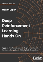
The next function calculates the value of the action from the state, using our transition, reward and values tables. We will use it for two purposes: to select the best action to perform from the state and to calculate the new value of the state on value iteration. Its logic is illustrated in the following diagram and we do the following:
- We extract transition counters for the given state and action from the transition table. Counters in this table have a form of dict, with target states as key and a count of experienced transitions as value. We sum all counters to obtain the total count of times we've executed the action from the state. We will use this total value later to go from an inpidual counter to probability.
- Then we iterate every target state that our action has landed on and calculate its contribution into the total action value using the Bellman equation. This contribution equals to immediate reward plus discounted value for the target state. We multiply this sum to the probability of this transition and add the result to the final action value.

Figure 8: The calculation of the state's value
In our diagram, we have an illustration of a calculation of value for state s and action a. Imagine that during our experience, we have executed this action several times ( ) and it ends up in one of two states,
  or
or  . How many times we have switched to each of these states is stored in our transition table as dict {:
 , : }. Then, the approximate value for the state and action Q(s, a) will be equal to the probability of every state, multiplied to the value of the state. From the Bellman equation, this equals to the sum of the immediate reward and the discounted long-term state value.
    def calc_action_value(self, state, action):
        target_counts = self.transits[(state, action)]
        total = sum(target_counts.values())
        action_value = 0.0
        for tgt_state, count in target_counts.items():
            reward = self.rewards[(state, action, tgt_state)]
            action_value += (count / total) * (reward + GAMMA * self.values[tgt_state])
        return action_value
The next function uses the function we just described to make a decision about the best action to take from the given state. It iterates over all possible actions in the environment and calculates value for every action. The action with the largest value wins and is returned as the action to take. This action selection process is deterministic, as the play_n_random_steps() function introduces enough exploration. So, our agent will behave greedily in regard to our value approximation.
    def select_action(self, state):
        best_action, best_value = None, None
        for action in range(self.env.action_space.n):
            action_value = self.calc_action_value(state, action)
            if best_value is None or best_value < action_value:
                best_value = action_value
                best_action = action
        return best_action
The play_episode function uses select_action to find the best action to take and plays one full episode using the provided environment. This function is used to play test episodes, during which we don't want to mess up with the current state of the main environment used to gather random data. So, we're using the second environment passed as an argument. The logic is very simple and should be already familiar to you: we just loop over states accumulating reward for one episode:
    def play_episode(self, env):
        total_reward = 0.0
        state = env.reset()
        while True:
            action = self.select_action(state)
            new_state, reward, is_done, _ = env.step(action)
            self.rewards[(state, action, new_state)] = reward
            self.transits[(state, action)][new_state] += 1
            total_reward += reward
            if is_done:
                break
            state = new_state
        return total_reward
The final method of the Agent class is our value iteration implementation and it is surprisingly simple, thanks to the preceding functions. What we do is just loop over all states in the environment, then for every state we calculate the values for the states reachable from it, obtaining candidates for the value of the state. Then we update the value of our current state with the maximum value of the action available from the state:
    def value_iteration(self):
        for state in range(self.env.observation_space.n):
            state_values = [self.calc_action_value(state, action)
                            for action in range(self.env.action_space.n)]
            self.values[state] = max(state_values)
That's all our agent's methods, and the final piece is a training loop and the monitoring of the code:
if __name__ == "__main__":
    test_env = gym.make(ENV_NAME)
    agent = Agent()
    writer = SummaryWriter(comment="-v-learning")
We create the environment we'll be using for testing, the Agent class instance and the summary writer for TensorBoard:
    iter_no = 0
    best_reward = 0.0
    while True:
        iter_no += 1
        agent.play_n_random_steps(100)
        agent.value_iteration()
The two lines in the preceding code snippet are the key piece in the training loop. First, we perform 100 random steps to fill our reward and transition tables with fresh data and then we run value iteration over all states. The rest of the code plays test episodes using the value table as our policy, then writes data into TensorBoard, tracks the best average reward, and checks for the training loop stop condition.
        reward = 0.0
        for _ in range(TEST_EPISODES):
            reward += agent.play_episode(test_env)
        reward /= TEST_EPISODES
        writer.add_scalar("reward", reward, iter_no)
        if reward > best_reward:
            print("Best reward updated %.3f -> %.3f" % (best_reward, reward))
            best_reward = reward
        if reward > 0.80:
            print("Solved in %d iterations!" % iter_no)
            break
    writer.close()
Okay, let's run our program:
rl_book_samples/Chapter05$ ./01_frozenlake_v_learning.py
[2017-10-13 11:39:37,778] Making new env: FrozenLake-v0
[2017-10-13 11:39:37,988] Making new env: FrozenLake-v0
Best reward updated 0.000 -> 0.150
Best reward updated 0.150 -> 0.500
Best reward updated 0.500 -> 0.550
Best reward updated 0.550 -> 0.650
Best reward updated 0.650 -> 0.800
Best reward updated 0.800 -> 0.850
Solved in 36 iterations!
Our solution is stochastic, and my experiments usually required from 12 to 100 iterations to reach a solution, but in all cases, it took less than a second to find a good policy that could solve the environment in 80% of runs. If you remember how many hours were required to achieve a 60% success ratio using Cross-entropy, then you can understand that this is a major improvement. There are several reasons for that.
First of all, the stochastic outcome of our actions, plus the length of the episodes (6-10 steps on average), makes it hard for the Cross-entropy method to understand what was done right in the episode and which step was a mistake. The value iteration works with inpidual values of state (or action) and incorporates the probabilistic outcome of actions naturally, by estimating probability and calculating the expected value. So, it's much simpler for the value iteration and requires much less data from the environment (which is called sample efficiency in RL).
The second reason is the fact that the value iteration doesn't need full episodes to start learning. In an extreme case, we can start updating our values just from the single example. However, for FrozenLake, due to the reward structure (we get 1 only after successfully reaching the target state), we still need to have at least one successful episode to start learning from a useful value table, which may be challenging to achieve in more complex environments. For example, you can try switching existing code to a larger version of FrozenLake, which has the name FrozenLake8x8-v0. The larger version of FrozenLake can take from 50 to 400 iterations to solve, and, according to TensorBoard charts, most of the time it waits for the first successful episode, then very quickly reaches convergence. The following is a chart with two lines. Orange corresponds to the reward during the training of FrozenLake-v0 (4x4) and blue is the reward of FrozenLake8x8-v0.:

Figure 9: The convergence of FrozenLake 4x4 and 8x8
Now it's time to compare the code that learns the values of states, as we just discussed, to the code that learns the values of actions.